
Below is an introduction to the terms, concepts and summary of the features of DOCSIS standard versions which i have compiled from several sources in an effort to learn about the cable broadband technology.
Cable Modem: is a device that is designed to bridge customer's home computing network to an external network, usually the Internet. This is accomplished by using the preexisting coaxial cable network, originally designed for the cable TV infrastructure, known as Community Antenna Television (CATV).
Coaxial Cable (RG-6 type): Many video channels, each carried at a specific frequency, are superimposed by the cable provider onto a single carrier medium - a standard coaxial cable. This process modulates each channel so that it is exactly 6 MHz (8MHz in Europe) away from the previous channel, and the frequency range available for a CATV provider to use typically runs from 42 to 850 MHz. When a user is watching a channel, the TV is tuned to the frequency that represents the channel and so displays only the part of the cable signal that corresponds to that channel. The legacy CATV infrastructure was designed as a one-way communication network.
ADSL: As demand for faster home internet service increased, cable companies began using their existing coax cable networks to offer digital internet connectivity. At the same time, telcos (phone companies) started using their existing copper two-wire phone lines to offer a similar service known as ADSL (Asynchronous Digital Subscriber Line), where the downstream connection is faster than the upstream connection. Unlike dialup, DSL uses a sophisticated frequency-modulation method to transmit data through copper line wires without disrupting the regular phone service over the line.
Quick comparison between Cable modem and ADSL broadband technologies:
| Cable Modem | ADSL |
|
| DSL is decent for browsing web, sending emails, sending and receiving pictures and downloading music but it usually lacks bandwidth for anything having to do with video. |
| Almost insensitive to distance between CMTS and CM as fiber optic cables can support digital data transmission over longer distances. | DSL is distance sensitive: the signal decreases with increasing distance between the modem and the network service provider, which results in a loss of data throughput. As a result, DSL modem may achieve only a fraction of the advertised data speeds. |
| Cable service operates on a coax cable which has a higher informational density and is physically thicker than phone wire. This provides a cleaner signal and allows you to modulate more data at higher frequencies with fewer errors. |
|
| Coax cable is a shared medium, meaning every house in the area around a local hub of coax (known as drop) is physically connected to the same coax cable. | A DSL home line is a dedicated connection that connects the home user directly with the service provider (the phone company). |
| Cable modems can upload faster than DSL modems can (max download speed being 38 Mbps and max upload speed being 30 Mbps) but the upstream bandwidth is usually limited by the ISP to a much slower rate. |
|
In short, i think the one can decide which of the two technologies to choose based on which one works out cheaper and/or reliable in their area as both these technologies are capable and can coexist as means to achieve broadband internet connection for home users. I used to use ADSL from airtel in India (Bangalore) and am using Cable modem from comcast in USA (Maynard, MA) and have noticed no significant difference in the service quality during video chats on internet (viz a scenario where high usage of upstream and downstream is made).
A Cable network:
A cable coax network is a bus topology - ie all service nodes (cable modems) are connected to a common medium, the coax bus. Each modem connected to a bus shares this line with every other modem when sending and receiving data. But generally cable modem networks use a technology called hybrid fiber coax (HFC), which incorporates both optical fiber along with coaxial cable to create a broadband network.


A fiber optic node has a broadband optical transmitter and receiver capable of converting the downstream optically modulated signal coming from the headend to an electrical signal going to the homes as well as electrical signals from the home into optical signals in the reverse path. Today, this downstream electrical output is a radio frequency modulated signal that ranges from 50 MHz to 1000 MHz. Fiber optic cables connect the optical node to a distant headend or hub in a point-to-point or star topology or in some cases, in a protected ring topology. The fiber optic node also contains a reverse path transmitter that sends communication from the home back to the headend. In the United States, this reverse signal is a modulated radio frequency ranging from 5 to 42 MHz while in other parts of the world, the range is 5 to 65 MHz.
The coaxial portion of the network connects 25 to 2000 homes (500 is typical) in a tree-and-branch configuration. Radio frequency amplifiers are used at intervals to overcome cable attenuation and passive losses caused by splitting or "tapping" the cable. Trunk coaxial cables are connected to the optical node and form a coaxial backbone to which smaller distribution cables connect. Trunk cables also carry AC power which is added to the cable line at usually either 60V or 90V by a power supply and a power inserter. The power is added to the cable line so that trunk and distribution amplifiers do not need an individual, external power source.
From the trunk cables, smaller distribution cables are connected to a port of the trunk amplifier to carry the RF signal and the AC power down individual streets. If needed, line extenders, which are smaller distribution amplifiers, boost the signals to keep the power of the television signal at a level that the TV can accept. The distribution line is then "tapped" into and used to connect the individual drops to customer homes. These taps pass the RF signal and block the AC power unless there are telephony devices that need the back-up power reliability provided by the coax power system. The tap terminates into a small coaxial drop using a standard screw type connector known as an “F” connector. The drop is then connected to the house where a ground block protects the system from stray voltages. Depending on the design of the network, the signal can then be passed through a splitter to multiple TVs and a cable modem.

A single downstream 6 MHz television channel may support up to 27 Mbps of downstream data throughput from the cable headend using 64 QAM (quadrature amplitude modulation) transmission technology. Speeds can be boosted to 36 Mbps using 256 QAM. Upstream channels may deliver 500 Kbps to 10 Mbps from homes using 16QAM or QPSK (quadrature phase shift key) modulation techniques, depending on the amount of spectrum allocated for service. This upstream and downstream bandwidth is shared by the active data subscribers connected to a given cable network segment, typically 500 to 2,000 homes on a modern HFC network.Most cable modem systems rely on a shared access platform, much like an office LAN. Because cable modem subscribers share available bandwidth during their sessions, there are concerns that cable modem users will see poor performance as the number of subscribers increases on the network. “Common sense dictates that 200 cable data subscribers sharing a 27-Mbps connection would each get only about 135 Kbps of throughput -- virtually the same speed as a 128-Kbps ISDN connection -- right? Not necessarily (Crockett, 99)”.
Unlike circuit-switched telephone networks where a caller is allocated a dedicated connection, cable modem users do not occupy a fixed amount of bandwidth during their online session. Instead, they share the network with other active users and use the network's resources only when they actually send or receive data in quick bursts. “So instead of 200 cable online users each being allocated 135 Kbps, they are able to grab all the bandwidth available during the millisecond they need to download their data packets -- up to many megabits per second (Fitzgerald, 99)”.
If congestion does begin to occur due to high usage, cable operators have the flexibility to add more bandwidth for data services. A cable operator can simply allocate an additional 6 MHz video channel for high-speed data, doubling the downstream bandwidth available to users. Another option for adding bandwidth is to subdivide the physical cable network by running fiber-optic lines deeper into neighborhoods. This reduces the number of homes served by each network segment, and thus, increases the amount of bandwidth available to end-users.
The cable modem access network operates at Layer 1 (physical) and Layer 2 (media access control/logical link control) of the Open System Interconnect (OSI) Reference Model. Thus, Layer 3 (network) protocols, such as IP traffic, can be seamlessly delivered over the cable modem platform to end-users. A cable modem has atleast two MAC addresses, one for the coax interface (aka HFC MAC) and one for the Ethernet interface (aka CMCI MAC for cable modem to CPE MAC).


The DOCSIS Standard:
Almost all cable modems available in retail stores are DOCSIS-certified, which means they can work on the network of any Internet service provider that supports DOCSIS (Data Over Cable Service Interface Specification). DOCSIS is a widely agreed-upon standard developed by a group of cable providers (MSOs - Multiple Service Operators). The company CableLabs runs a certification program for hardware vendors who manufacture DOCSIS-compatible equipment.
The physical hardware of a cable modem includes, a CPU, chipset, RAM and flash memory. There are only a few DOCSIS-compatible microcontrollers in the market - major manufacturers being Broadcom and Texas Instruments.
The DOCSIS standard covers every aspect of cable modem infrastructure - from CM (cable modem at customer premise) to operator's headend equipment (CMTS). This specification details many of the basic functions of the customer's cable modem,
- including how frequencies are modulated on the coax cable,
- how the SNMP protocol applies to the cable modem,
- how data is sent and received,
- how the modem should network with CMTS, and
- how privacy is initiated.
Due to this standardization, consumers can purchase off-the-shelf retail modems for use with many different service providers, and cable operators can deploy newer and more innovative services to consumers.
As QAM level increases, the points that represent symbols have to be placed closer together and are then more difficult to distinguish from one another because of line noise, which creates a higher error rate. Cable modems use an entire TV channel's worth of bandwidth (6MHz for NTSC) for their downstream data. Because of the combined upstream noise from ingress (the distortion created when frequencies enter a medium), the upstream symbol rate is less than the downstream, which has no combined ingress noise issues.
To detect and troubleshoot network problems, cable engineers examine packet error statistics. Each time a cable modem detects a packet error, it will record it. By comparing the total number of received packets with the erroneous ones, the cable modem will produce what's known as the codeword error rate (CER).
NonErr - docsIfCmtsCmStatusUnerroreds
CorrErr - docsIfCmtsCmStatusCorrecteds
UnCorr - docsIfCmtsCmStatusUncorrectables
CER (%) = 100*(UnCorr/(NonErr+CorrErr+UnCorr))
Error ratios higher than 1% should trigger CM maintenance. Formula as mentioned here.
How modems register online?
DOCSIS specification details the procedure a modem should follow in order to register on the cable network - called provisioning process. Across DOCSIS versions, the registration process is same.
1. Tune: When a modem is powered on for the first time, it has no prior knowledge of the cable system it may be connected to. It creates a large frequency scan list for the region for which the modem was designated, which is also known as frequency plan (There are 4 major regions - North America, Europe, China, Japan and each use different channel frequencies so the modem only needs to have a list of frequencies of its intended region of use). With the list retrieved, modem begins to search for a downstream frequency from the list to connect to.
A modem scans for frequencies until it locks on to one. Since a single coax cable can contain multiple digital services, it is up to the CMTS to determine if the new device (the modem performing frequency scan) is supposed to access that particular frequency. This is accomplished by checking the modem's MAC address. Once a modem has locked on to the download channel, it proceeds to obtain the upstream parameters by listening for special packets known as UCDs (Upstream channel descriptors), which contain the transmission parameters for the upstream channel.
2. Range: Once both downstream and upstream channels are synched, the modems makes minor ranging adjustments. Ranging is the process of determining network latency (the time it takes for the data to travel) between cable modem and CMTS. A ranging request (RNG-REQ) must be transmitted from cable modem to CMTS upon registering and periodically there-after. Once the CMTS receives a ranging request, it sends the cable modem a ranging response (RNG-RSP) that contains timing, power, and frequency adjustment information for the cable modem to use. Ranging offset is the delay correction applied by the modem to help synchronize its upstream transmissions.
3. Connect: Next the cable modem must establish IP Connectivity. To do this, it sends a DHCP discover packet and listens for a DHCP offer packet. A DHCP server must be set up at the headend to offer this service, such as Cisco Network Registrar (CNR) or similar. The DHCP offer packet contains IP setup parameters for the cable modem, which includes the HFC IP address, the TFTP service IP address, the boot file name (aka the TFTP config) and the time server's IP address.
4. Configure: After this is done, the modem can (optionally) use the IP protocol to establish the current time of day (TOD) from a Unix type time server running at the headend.
Now the modem must connect to the TFTP server and request the boot file. The boot file contains many important parameters, such as downstream and upstream speed settings (DOCSIS 1.0 only), SNMP settings, and various other network settings. The TFTP server is usually a service that runs in the CMTS.
5. Register: Once the modem downloads the config file, it processes it. It then sends an exact copy of the config file back to the CMTS server, a process known as transferring the operational parameters. This part of registration process is also used to authenticate the modem. If the modem is listed in the CMTS database as valid, the modem receives a message from the CMTS that it has passed registration.
At this stage, the modem has been authenticated and is allowed to initialize its baseline privacy, an optional step that permits modem to initiate privacy features that allow it to encrypt and decrypt its own network traffic to and from the CMTS. The encryption is based on the private digital certificate (X.509 standard) that is installed on the modem prior to registration.
Finally the modem connects to cable operator's internet backbone, and is allowed to access the Web. The cable modem is now operational.

Versions of DOCSIS:
DOCSIS 1.0 key features:
- 10Mbps upstream capability
- 40Mbps downstream capability
- Bandwidth efficient through use of variable packet lengths
- Class of service (CoS) support
- CMTS upstream and downstream limitations
- Extensions for security (BPI)
- QPSK and QAM modulation formats
- SNMP v2c
DOCSIS 1.1 key features: Focused more on security. No hardware requirement changed so many DOCSIS 1.0 certified modems were able to use this 1.1 versio with just a simple firmware upgrade.
- Baseline privacy interface plus (BPI+)
- MAC collision detection to prevent cable modem cloning
- Service flows that allow for tiered services
- SNMP v3
- VoIP support
DOCSIS 2.0 key features: focuses more on data-over-coax technology. Using Advanced TDMA (A-TDMA), this spec allows cable modems to be upstream capable of up to 30Mbps while previous releases allow up to 10Mbps only. This higher bandwidth allows providers to offer consumers two-way video services, such as video phone service. However, this new standard requires consumer modem upgrade because earlier modem hardware is not capable of this faster upload speed.
DOCSIS 3.0 focuses on data speed improvements to both upstream and downstream channels, as well as many innovations for services other than Internet. These enhancements are accomplished by bridging multiple channels together at the same time, also known as channel bonding. Thus a bandwidth of 200Mbps for downstream and 100Mbps for upstream will be possible. Additional features include support for IPv6.
So that's in short about the cable broadband technology. The DOCSIS 3.0 standard is slated to capture only 60% of the cable market by 2011. The first few products which comply with 3.0 will be released this year 2007 sometime. I have collected the above information from various sources noteable among them being wikipedia and "Hacking the Cable Modem: What Cable companies don't want you to know" book by DerEngel, a very readable work on the cable modem internals.
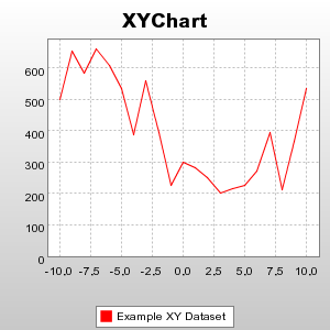 I recently had an opportunity to use the Cewolf 1.0 at work for some Time Series plots (a variant of the XY Chart, shown in the figure above, where the X-axis is for time values). This blog is about Cewolf and how to create time series plots with it.


